Reproducible Reporting
Last updated on 2026-05-05 | Edit this page
Estimated time: 60 minutes
Overview
Questions
- How do I combine my analysis and write-up in one document?
- What is R Markdown and why is it better than copy-pasting from SPSS output?
- How do I create a report that updates when data changes?
Objectives
- Create an R Markdown document that combines text, code, and output
- Generate tables and figures that update automatically
- Export reports to Word, PDF, or HTML
- Understand why script-based reporting is more reliable than SPSS output export
The problem with copy-paste
If you have used SPSS for reporting, this workflow will feel very familiar:
- Run your analysis in SPSS
- Get a table or chart in the Output window
- Copy it
- Paste it into your Word document
- Write your interpretation around it
- Your supervisor / colleague sends updated data
- Go back to step 1 and redo everything
This copy-paste workflow is fragile. Every time the data changes, you need to re-run every analysis, re-copy every table, and re-paste into your document. Along the way, it is easy to accidentally paste an old table, forget to update a number in the text, or lose track of which version of the analysis matches your report.
R Markdown solves this problem. It lets you write your text and your analysis in a single file. When the data changes, you press one button and the entire report — text, tables, figures, and all the numbers in your sentences — updates automatically.
This is not just convenience — it is research integrity
When your numbers and your text live in the same document, it is physically impossible for them to get out of sync. This matters for policy reports, academic papers, and any situation where someone else relies on your numbers.
R Markdown basics
An R Markdown file is a plain text file with the extension
.Rmd. It has three types of content:
- A YAML header at the top (metadata about the document)
- Markdown text (your writing)
- Code chunks (your R analysis)
Let us look at each one.
The YAML header
Every R Markdown document starts with a block between
--- lines. This is the YAML header, and it controls the
document settings:
---
title: "Aruba Tourism Analysis Q1 2023"
author: "Your Name"
date: "2026-04-22"
output: word_document
---
The output line controls the format of your final
document:
| Output format | What you get |
|---|---|
word_document |
A .docx Word file |
html_document |
A web page |
pdf_document |
A PDF (requires LaTeX) |
For most government and policy work, word_document is
the most practical choice — your colleagues can open it, comment on it,
and print it without installing anything.
Start with Word, explore later
We recommend word_document for this course because it
fits the workflow most SPSS users already have. Once you are
comfortable, try html_document — it supports interactive
tables and plots.
Markdown text formatting
Between your code chunks, you write normal text using Markdown — a simple way to format text with plain characters. Here are the essentials:
# First-level heading
## Second-level heading
### Third-level heading

**bold text**
*italic text*

- Bullet point one
- Bullet point two

1. Numbered item one
2. Numbered item two

[Link text](https://example.com)
That is all you need for most reports. If you have used WhatsApp or Slack formatting, this will feel familiar.
Code chunks
A code chunk is where your R code lives. It starts with
```{r} and ends with ```:
```{r}
library(tidyverse)
visitors <- read_csv("data/aruba_visitors.csv")
summary(visitors$visitors_stayover)
```
When you knit the document, R runs the code and places the output directly into your report. No copying, no pasting.
Chunk options
You can control what appears in the final document by adding options to the chunk header:
```{r, echo = FALSE, message = FALSE, warning = FALSE}
library(tidyverse)
visitors <- read_csv("data/aruba_visitors.csv")
```| Option | What it does |
|---|---|
echo = FALSE |
Hides the code, shows only the output |
message = FALSE |
Suppresses package loading messages |
warning = FALSE |
Suppresses warnings |
eval = FALSE |
Shows the code but does not run it |
fig.width = 8 |
Sets figure width in inches |
fig.height = 5 |
Sets figure height in inches |
For a polished report aimed at a non-technical audience, you will
typically set echo = FALSE so readers see results but not
code.
Inline R code
This is the feature that makes R Markdown truly powerful. You can embed R calculations directly inside your sentences:
The dataset contains `r nrow(visitors)` observations.When knitted, this becomes:
The dataset contains 168 observations.
If the data changes and you re-knit, that number updates automatically. No more manually searching through your Word document to find every number that needs updating.
Knitting: from .Rmd to a finished document
To turn your .Rmd file into a Word document (or HTML, or
PDF), you knit it. In RStudio:
- Click the Knit button at the top of the editor (the ball of yarn icon)
- R runs all your code chunks from top to bottom in a clean environment
- The finished document appears
The most common issue learners face is that knitting fails because
the .Rmd file does not load packages or data that earlier
chunks depend on. Remind participants that knitting starts from a
blank environment — every package and dataset must be
loaded within the .Rmd file itself, even if it is already
loaded in their current R session.
Another common issue: file paths. If participants use
read_csv("data/aruba_visitors.csv"), the working directory
during knitting is the folder where the .Rmd file is saved.
Make sure the data file is in the right relative location.
Knitting runs everything fresh
A common mistake is to rely on objects you created in your R console
but never included in the .Rmd file. When you knit, R
starts with a completely empty workspace. If you get an error like
“object not found,” it usually means you forgot to include the code that
creates that object in your .Rmd file.
Building a mini-report
Let us build a short tourism analysis report step by step. In RStudio:
- Go to File > New File > R Markdown…
- Enter a title like “Aruba Tourism Report”
- Enter your name as author
- Select Word as the default output format
- Click OK
RStudio gives you a template document. Delete everything below the YAML header and replace it with the following sections.
Step 1: Setup chunk
The first code chunk in any report should load your packages and data. We hide the code and messages because the reader does not need to see them.
R
# This would be at the top of your .Rmd file (after the YAML header):

# ```{r setup, message = FALSE, warning = FALSE, echo = FALSE}
library(tidyverse)
visitors <- read_csv("data/aruba_visitors.csv")
# ```
Step 2: Write an introduction in Markdown
Below the setup chunk, write some context in plain Markdown:
## Introduction

This report summarizes visitor arrivals to Aruba for the period
2019--2023. Data are drawn from quarterly records of stay-over
and cruise visitors by country of origin.
Step 3: A summary table
Now add a code chunk that produces a summary table. The
knitr::kable() function turns a data frame into a nicely
formatted table in your output document:
R
visitors <- read_csv("data/aruba_visitors.csv")

annual_summary <- visitors |>
  group_by(year) |>
  summarise(
    total_stayover = sum(visitors_stayover),
    total_cruise = sum(visitors_cruise),
    avg_spending = round(mean(avg_spending_usd), 0),
    avg_satisfaction = round(mean(satisfaction_score), 1)
  )

knitr::kable(annual_summary, col.names = c(
  "Year", "Stay-over Visitors", "Cruise Visitors",
  "Avg Spending (USD)", "Avg Satisfaction"
))
| Year | Stay-over Visitors | Cruise Visitors | Avg Spending (USD) | Avg Satisfaction |
|---|---|---|---|---|
| 2019 | 440650 | 195950 | 919 | 7.7 |
| 2020 | 208480 | 61200 | 821 | 7.3 |
| 2021 | 357200 | 121080 | 888 | 7.5 |
| 2022 | 443700 | 203720 | 924 | 7.8 |
| 2023 | 463700 | 213020 | 938 | 7.8 |
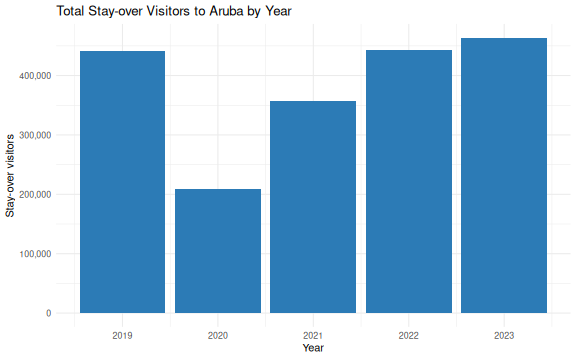
Step 4: A visualization
Add another chunk with a ggplot2 chart:
R
visitors <- read_csv("data/aruba_visitors.csv")

annual_stayover <- visitors |>
  group_by(year) |>
  summarise(total_stayover = sum(visitors_stayover))

ggplot(annual_stayover, aes(x = year, y = total_stayover)) +
  geom_col(fill = "#2c7bb6") +
  scale_y_continuous(labels = scales::comma) +
  labs(
    title = "Total Stay-over Visitors to Aruba by Year",
    x = "Year",
    y = "Stay-over visitors"
  ) +
  theme_minimal()
Step 5: Interpretation with inline R
Now write a paragraph that uses inline R to insert numbers directly:
In your .Rmd file, you would write something like
this:
The strongest year for stay-over tourism was `r best_year$year`,
with `r scales::comma(best_year$total_stayover)` visitors.
The weakest year was `r worst_year$year`, with
`r scales::comma(worst_year$total_stayover)` visitors.
When knitted, this becomes a complete sentence with real numbers — numbers that update automatically if the data ever changes.
Step 6: Knit
Click the Knit button. RStudio generates a Word document with your introduction, table, chart, and interpretation — all in one step, all from one file.
Compare this to the SPSS workflow
Think about what you just did: you loaded data, computed a summary, created a chart, and wrote an interpretation with automatically-calculated numbers — all in a single file. If the data file is updated next quarter, you re-knit and the entire report updates. No manual copy-paste. No version confusion.
A complete example
Here is what a minimal but complete .Rmd file looks
like, all in one place:
---
title: "Aruba Tourism Quarterly Report"
author: "Your Name"
date: "`r Sys.Date()`"
output: word_document
---

```{r setup, message = FALSE, warning = FALSE, echo = FALSE}
library(tidyverse)
visitors <- read_csv("data/aruba_visitors.csv")
```

## Overview

This report summarizes Aruba visitor statistics for 2019--2023.

```{r summary-table, echo = FALSE}
annual <- visitors |>
  group_by(year) |>
  summarise(
    stayover = sum(visitors_stayover),
    cruise = sum(visitors_cruise)
  )

knitr::kable(annual, col.names = c("Year", "Stay-over", "Cruise"))
```

```{r trend-chart, echo = FALSE, fig.width = 7, fig.height = 4}
ggplot(annual, aes(x = year, y = stayover)) +
  geom_line(linewidth = 1, colour = "#2c7bb6") +
  geom_point(size = 3, colour = "#2c7bb6") +
  scale_y_continuous(labels = scales::comma) +
  labs(title = "Stay-over Visitors by Year", x = "Year", y = "Visitors") +
  theme_minimal()
```

## Key Findings

```{r findings, echo = FALSE}
latest <- annual |> filter(year == max(year))
previous <- annual |> filter(year == max(year) - 1)
change_pct <- round((latest$stayover - previous$stayover) /
                       previous$stayover * 100, 1)
```

In `r latest$year`, Aruba received
`r scales::comma(latest$stayover)` stay-over visitors, a
`r change_pct`% change compared to the previous year.
Challenge 1: Create a tourism report
Create a new R Markdown document (File > New File > R Markdown) and build a short report that does the following:
- Loads
data/aruba_visitors.csv - Produces a summary table showing average spending and
satisfaction by country of origin (using
knitr::kable()) - Creates a bar chart of average spending by origin
- Includes at least one inline R value in a written interpretation sentence (for example, which origin market has the highest average spending)
- Knits to Word
Here is one way to approach it. Your file would look like this:
---
title: "Aruba Visitor Spending by Origin"
author: "Your Name"
date: "`r Sys.Date()`"
output: word_document
---

```{r setup, message = FALSE, warning = FALSE, echo = FALSE}
library(tidyverse)
visitors <- read_csv("data/aruba_visitors.csv")
```

## Visitor Spending by Country of Origin

```{r origin-table, echo = FALSE}
origin_summary <- visitors |>
  group_by(origin) |>
  summarise(
    avg_spending = round(mean(avg_spending_usd), 0),
    avg_satisfaction = round(mean(satisfaction_score), 1)
  ) |>
  arrange(desc(avg_spending))

knitr::kable(origin_summary, col.names = c(
  "Origin", "Avg Spending (USD)", "Avg Satisfaction"
))
```

```{r origin-chart, echo = FALSE, fig.width = 7, fig.height = 4}
ggplot(origin_summary, aes(x = reorder(origin, avg_spending),
                            y = avg_spending)) +
  geom_col(fill = "#2c7bb6") +
  coord_flip() +
  labs(
    title = "Average Visitor Spending by Country of Origin",
    x = "Country of Origin",
    y = "Average Spending (USD)"
  ) +
  theme_minimal()
```

## Interpretation

```{r top-spender, echo = FALSE}
top <- origin_summary |> slice(1)
```

The highest-spending visitor segment is from `r top$origin`,
with an average spend of $`r top$avg_spending` USD per trip.
This group also has an average satisfaction score of
`r top$avg_satisfaction` out of 10.
Capstone: a full report from one command
The capstone of this course is a single R Markdown file that produces a polished, self-contained HTML report at the press of the Knit button. The worked example is the Xander Bogaerts baseball statistics report you saw in Episode 1’s opening — the same file, opened now with the skills from this episode in hand.
Pull the template and its stylesheet from the course repository on the University of Aruba’s GitHub into your workshop folder:
R
# Iteration: 1
base <- "https://raw.githubusercontent.com/University-of-Aruba/r-for-spss-users/main/episodes/files"

download.file(file.path(base, "xander-bogaerts-report-template.Rmd"),
              "xander-bogaerts-report-template.Rmd")
download.file(file.path(base, "xander-report.css"),
              "xander-report.css")

file.edit("xander-bogaerts-report-template.Rmd")
Both files land next to each other in the working directory, which is all the knit step needs. Walk through the template’s structure: a YAML header, a hidden setup chunk, a small number of analysis chunks, and prose with inline R for the narrative numbers. Everything above in this episode is inside that template — the capstone is assembly, not new material.
- R Markdown combines your analysis and write-up in a single document
- When data changes, re-knitting updates every table and figure automatically
- You can output to Word, PDF, or HTML from the same source file
- This eliminates the copy-paste errors that are common with SPSS output