Reproducible Reporting

Last updated on 2026-09-29 | Edit this page

Overview

Questions

How do I combine my analysis and write-up in one document?
What is R Markdown and why is it better than copy-pasting from SPSS output?
How do I create a report that updates when data changes?

Objectives

Create an R Markdown document that combines text, code, and output
Generate tables and figures that update automatically
Export reports to Word, PDF, or HTML
Understand why script-based reporting is more reliable than SPSS output export

Cartoon of a researcher pressing one button on a machine that turns a changed squad list into a finished report

Callout

If your files are not where R expects them

The report code below reads data/blue_wave_squad.csv, which assumes the file sits in a data folder next to your report. If that is not your situation this morning, put this line at the top of the report instead and change each read_csv() to match:

R

base <- "https://raw.githubusercontent.com/University-of-Aruba/blue-wave-analytics/main/episodes/data/"
squad <- read_csv(paste0(base, "blue_wave_squad.csv"))

A report that reads from a URL is still reproducible, and it has one advantage for a report you send to someone else: it carries its own data with it. The trade-off is that it needs a connection and it breaks if the file moves.

The problem with copy-paste

If you have used SPSS for reporting, this workflow will feel familiar:

Run your analysis in SPSS
Get a table or chart in the Output window
Copy it
Paste it into your Word document
Write your interpretation around it
A colleague sends updated data
Go back to step 1 and redo everything

This workflow is fragile. Every time the data changes you re-run every analysis, re-copy every table, and re-paste into your document. Along the way it is easy to paste an old table, forget to update a number in the text, or lose track of which version of the analysis matches your report.

R Markdown solves this. It lets you write your text and your analysis in a single file. When the data changes you press one button and the entire report, text, tables, figures, and all the numbers inside your sentences, updates.

Callout

This is a research integrity question, not only a convenience

When your numbers and your text live in the same document, it is physically impossible for them to drift apart. That matters for policy reports, academic papers, and any situation where someone else relies on your numbers.

It matters more when the numbers are about people. The squad dataset behind this course is scraped from Wikipedia squad tables that are edited continuously, and two players in it have no club listed at all. A report that hard-codes “87 percent play abroad” into a Word file loses that context the moment the file leaves your hands, and is quietly wrong the next time a squad is called. A report that computes the figure at knit time can carry the caveat with it, and update both together.

R Markdown basics

An R Markdown file is a plain text file with the extension .Rmd. It has three types of content:

A YAML header at the top, metadata about the document
Markdown text, your writing
Code chunks, your R analysis

The YAML header

Every R Markdown document starts with a block between --- lines. This is the YAML header, and it controls the document settings:

---
title: "Curaçao Squad Report 2026"
author: "Your Name"
date: "2026-09-15"
output: word_document
---

The output line controls the format of your final document:

Output format	What you get
`word_document`	A .docx Word file
`html_document`	A web page
`pdf_document`	A PDF (requires LaTeX)

For most government and policy work word_document is the most practical choice. Your colleagues can open it, comment on it, and print it without installing anything.

Callout

Start with Word, explore later

We recommend word_document for this course because it fits the workflow most SPSS users already have. Once you are comfortable, try html_document. It supports interactive tables and plots, and it is what the capstone report at the end of this episode uses.

Markdown text formatting

Between your code chunks you write normal text using Markdown, a simple way to format text with plain characters:

# First-level heading
## Second-level heading
### Third-level heading

**bold text**
*italic text*

- Bullet point one
- Bullet point two

1. Numbered item one
2. Numbered item two

[Link text](https://example.com)

That is all you need for most reports. If you have used WhatsApp or Slack formatting, this will feel familiar.

Code chunks

A code chunk is where your R code lives. It starts with ```{r} and ends with ```:

```{r}
library(tidyverse)
squad <- read_csv("data/blue_wave_squad.csv")
table(squad$team_code)
```

When you knit the document, R runs the code and places the output directly into your report. No copying, no pasting.

Chunk options

You control what appears in the final document by adding options to the chunk header:

```{r, echo = FALSE, message = FALSE, warning = FALSE}
library(tidyverse)
squad <- read_csv("data/blue_wave_squad.csv")
```

Option	What it does
`echo = FALSE`	Hides the code, shows only the output
`message = FALSE`	Suppresses package loading messages
`warning = FALSE`	Suppresses warnings
`eval = FALSE`	Shows the code but does not run it
`fig.width = 8`	Sets figure width in inches
`fig.height = 5`	Sets figure height in inches

For a polished report aimed at a non-technical audience you will typically set echo = FALSE so readers see results but not code.

Callout

`warning = FALSE` is not a fix

It is tempting to put warning = FALSE on every chunk so the report looks clean. Remember what the warnings in Episode 4 were telling you: rows dropped because of missing values. Suppressing the warning does not stop the rows being dropped, it stops you finding out.

Set warning = FALSE at the end, once you have read every warning and know why each one is there. Not at the start, to make them go away.

Inline R code

This is the feature that makes R Markdown powerful. You can embed R calculations directly inside your sentences:

The dataset contains `r nrow(squad)` players.

When knitted, this becomes:

The dataset contains 94 players.

If the data changes and you re-knit, that number updates. No more searching through a Word document for every number that needs correcting.

Knitting: from .Rmd to a finished document

To turn your .Rmd file into a Word document, or HTML, or PDF, you knit it. In RStudio:

Click the Knit button at the top of the editor, the ball of yarn icon
R runs all your code chunks from top to bottom in a clean environment
The finished document appears

Callout

Knitting runs everything fresh

A common mistake is to rely on objects you created in your R console but never included in the .Rmd file. When you knit, R starts with a completely empty workspace. If you get an error like “object not found”, it usually means you forgot to include the code that creates that object in your .Rmd file.

Building a mini-report

Let us build a short squad analysis report step by step. In RStudio:

Go to File > New File > R Markdown…
Enter a title like “Curaçao Squad Report”
Enter your name as author
Select Word as the default output format
Click OK

RStudio gives you a template document. Delete everything below the YAML header and replace it with the following sections.

Step 1: Setup chunk

The first code chunk in any report should load your packages and data. We hide the code and messages because the reader does not need to see them.

R

# This would be at the top of your .Rmd file, after the YAML header:

# ```{r setup, message = FALSE, warning = FALSE, echo = FALSE}
library(tidyverse)
squad <- read_csv("data/blue_wave_squad.csv")
# ```

Step 2: Write an introduction in Markdown

Below the setup chunk, write some context in plain Markdown:

## Introduction

This report summarises where the players called up to the four ABC
island national squads play their club football, using squad lists
compiled in 2026.

Step 3: A summary table

Now add a code chunk that produces a summary table. The knitr::kable() function turns a data frame into a formatted table in your output document:

R

squad <- read_csv("data/blue_wave_squad.csv") |>
  mutate(
    island = if_else(str_starts(team_code, "CUW"), "Curaçao", "Aruba"),
    gender = if_else(str_ends(team_code, "M"), "Men", "Women"),
    based_abroad = !(club_country %in% c("CUW", "ABW", "X"))
  )

squad_summary <- squad |>
  group_by(island, gender) |>
  summarise(
    players    = n(),
    abroad     = sum(based_abroad),
    pct_abroad = round(100 * mean(based_abroad)),
    in_nld     = sum(club_country == "NLD"),
    .groups = "drop"
  ) |>
  arrange(desc(pct_abroad))

knitr::kable(squad_summary, col.names = c(
  "Island", "Squad", "Players", "Abroad", "% abroad", "In Netherlands"
))

Island	Squad	Players	Abroad	% abroad	In Netherlands
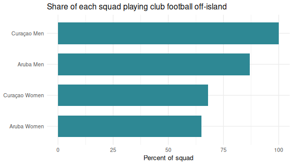
Curaçao	Men	26	26	100	10
Aruba	Men	23	20	87	18
Curaçao	Women	22	15	68	12
Aruba	Women	23	15	65	14

Step 4: A visualization

Add another chunk with a ggplot2 chart:

R

ggplot(squad_summary, aes(x = reorder(paste(island, gender), pct_abroad),
                          y = pct_abroad)) +
  geom_col(fill = "#2e8894", width = 0.7) +
  coord_flip() +
  labs(
    title = "Share of each squad playing club football off-island",
    x = NULL,
    y = "Percent of squad"
  ) +
  theme_minimal(base_size = 13)

Step 5: Interpretation with inline R

Inline R can only use objects that already exist when knitr reaches the sentence. So first add a chunk that picks out the squads with the highest and lowest share of players abroad from the squad_summary table you built in Step 3:

R

most  <- squad_summary |> slice_max(pct_abroad, n = 1)
least <- squad_summary |> slice_min(pct_abroad, n = 1)

In your own report, set echo = FALSE on this chunk so the reader sees only the sentence. Then, below the chunk and outside it, write the paragraph in plain Markdown with the inline R in it:

The squad most dependent on players based overseas is the
`r paste(most$island, most$gender)` team, at
`r most$pct_abroad`%. The least dependent is
`r paste(least$island, least$gender)`, at
`r least$pct_abroad`%.

When knitted this becomes a complete sentence with real numbers, numbers that update if the data ever changes.

Step 6: Knit

Click the Knit button. RStudio generates a Word document with your introduction, table, chart, and interpretation, in one step, from one file.

Callout

Compare this to the SPSS workflow

You loaded data, computed a summary, created a chart, and wrote an interpretation with automatically calculated numbers, all in a single file. If the squad list is updated after the next international window, you re-knit and the entire report updates. No manual copy-paste. No version confusion.

A complete example

Here is what a minimal but complete .Rmd file looks like, all in one place:

---
title: "ABC Islands Squad Report"
author: "Your Name"
date: "`r Sys.Date()`"
output: word_document
---

```{r setup, message = FALSE, warning = FALSE, echo = FALSE}
library(tidyverse)
squad <- read_csv("data/blue_wave_squad.csv") |>
  mutate(
    island = if_else(str_starts(team_code, "CUW"), "Curaçao", "Aruba"),
    based_abroad = !(club_country %in% c("CUW", "ABW", "X"))
  )
```

## Overview

This report summarises where the 2026 ABC island national squads play.

```{r summary-table, echo = FALSE}
by_island <- squad |>
  group_by(island) |>
  summarise(players = n(), abroad = sum(based_abroad))

knitr::kable(by_island, col.names = c("Island", "Players", "Abroad"))
```

```{r composition-chart, echo = FALSE, fig.width = 7, fig.height = 4}
ggplot(squad, aes(x = team_code, fill = club_country)) +
  geom_bar(position = "fill") +
  scale_y_continuous(labels = scales::percent) +
  labs(title = "Squad composition by club country", x = NULL, y = NULL) +
  theme_minimal()
```

## Key findings

```{r findings, echo = FALSE}
cuw <- by_island |> filter(island == "Curaçao")
aru <- by_island |> filter(island == "Aruba")
gap <- round(100 * (cuw$abroad / cuw$players - aru$abroad / aru$players))
```

Curaçao fields `r cuw$abroad` of
`r cuw$players` players from clubs off the island, against
`r aru$abroad` of `r aru$players` for
Aruba, a gap of `r gap` percentage points.

Challenge

Challenge 1: Create a squad report

Create a new R Markdown document, File > New File > R Markdown, and build a short report that does the following:

Loads data/blue_wave_squad.csv
Produces a summary table showing the number of players by position and club country for one squad of your choice, using knitr::kable()
Creates a bar chart of club country for that squad
Includes at least one inline R value in a written interpretation sentence
Knits to Word

Show me the solution

One way to approach it. Your file would look like this:

---
title: "Curaçao Men's Squad, 2026"
author: "Your Name"
date: "`r Sys.Date()`"
output: word_document
---

```{r setup, message = FALSE, warning = FALSE, echo = FALSE}
library(tidyverse)
squad <- read_csv("data/blue_wave_squad.csv")
this <- filter(squad, team_code == "CUW-M")
```

## Squad composition

```{r position-table, echo = FALSE}
knitr::kable(table(this$position, this$club_country))
```

```{r country-chart, echo = FALSE, fig.width = 7, fig.height = 4}
this |>
  filter(club_country != "X") |>
  count(club_country, sort = TRUE) |>
  ggplot(aes(x = reorder(club_country, n), y = n)) +
  geom_col(fill = "#2e8894") +
  coord_flip() +
  labs(title = "Club country", x = NULL, y = "Players") +
  theme_minimal()
```

## Interpretation

```{r top-country, echo = FALSE}
top <- this |>
  filter(club_country != "X") |>
  count(club_country, sort = TRUE) |>
  slice(1)
unknown <- sum(this$club_country == "X")
```

The largest single destination is `r top$club_country`,
which accounts for `r top$n` of the
`r nrow(this)` players called up.
`r unknown` players could not be placed at a club and are
excluded from the chart above.

Note the last sentence. The exclusion is written into the report by the same code that performs it, so the two can never disagree.

Capstone: a full report from one command

The capstone of this course is a single R Markdown file that produces a polished, self-contained report at the press of the Knit button. The worked example is the squad report you saw in Episode 1’s opening, opened now with the skills from this episode in hand.

Pull the template and its stylesheet from the course repository into your workshop folder:

R

# Iteration: 1
base <- "https://raw.githubusercontent.com/University-of-Aruba/blue-wave-analytics/main/episodes/files"

download.file(file.path(base, "blue-wave-squad-report-template.Rmd"),
              "blue-wave-squad-report-template.Rmd")
download.file(file.path(base, "blue-wave-report.css"),
              "blue-wave-report.css")

file.edit("blue-wave-squad-report-template.Rmd")

Both files land next to each other in the working directory, which is what the knit step needs. The template expects the data in a data subfolder, which is where you put it in Episode 2.

Walk through its structure: a YAML header with a params block, a hidden setup chunk, a handful of analysis chunks, and prose with inline R for the narrative numbers. Everything above in this episode is inside that template. The capstone is assembly, not new material.

Callout

One template, four reports

Look at the top of the template:

YAML

params:
  team: "CUW-M"
  data_dir: "data"
  squad_file: "blue_wave_squad.csv"

Every reference to a specific squad inside the document goes through params$team. Change that one line to "ARU-W", knit again, and you get the Aruba women’s report: different numbers, different charts, different sentences, same file.

This is the idea the whole course has been building toward. You have not written a report. You have written a thing that writes reports.

New squad, same report

Everything you have computed since Wednesday comes from the squad Curaçao took to the World Cup in June. On 11 September the national team named a new one for the Nations League window: eight of those twenty-six are out and five players are new. In the SPSS workflow at the top of this episode, that is step 7. Go back to step 1.

Here it is one download and one changed line. The new call-up sits in the course repository as a second file, next to the one you already have:

R

# Iteration: 1
download.file(
  "https://raw.githubusercontent.com/University-of-Aruba/blue-wave-analytics/main/episodes/data/blue_wave_squad_2026-09.csv",
  "data/blue_wave_squad_2026-09.csv"
)

Open the template, change squad_file in the header to "blue_wave_squad_2026-09.csv", and knit. Or leave the file alone and pass the new value in from the console, which also keeps the first report instead of overwriting it:

R

rmarkdown::render(
  "blue-wave-squad-report-template.Rmd",
  params = list(squad_file = "blue_wave_squad_2026-09.csv"),
  output_file = "curacao-men-2026-09.html"
)

Put the two reports side by side. The cover figures, every sentence with a number in it, the charts, the chi-square in the callout and the squad table at the bottom have all been recomputed. Nobody retyped anything.

Challenge

Challenge 2: What moved, and what held?

Compare the two Curaçao men’s reports. Which figures changed? Is it still true that no player in the squad plays club football on the island? Does the gender result from Episode 5 survive the new call-up?

Show me the solution

The squad went from 26 players to 23 and now spans 11 countries instead of 10. The Netherlands share fell from 38 percent of the squad to 30. Not one player is at a club on Curaçao, in either call-up. The gender test holds (p = 0.008, against 0.006 before) and the island comparison is still null.

The finding was about dispersion, and the new squad is more dispersed than the old one. One re-run will not tell you whether that is a trend. It does tell you that the claim did not depend on one particular squad list.

Callout

The list that was right on Wednesday

The region code you wrote in Episode 3 names the European countries one by one. Run it on the new file and look at what the .default line caught:

R

squad_new <- read_csv("data/blue_wave_squad_2026-09.csv") |>
  mutate(
    island    = if_else(str_starts(team_code, "CUW"), "Curaçao", "Aruba"),
    home_code = if_else(island == "Curaçao", "CUW", "ABW"),
    region = case_when(
      club_country == "X"       ~ "Unknown",
      club_country == home_code ~ "Home island",
      club_country == "NLD"     ~ "Netherlands",
      club_country == "USA"     ~ "North America",
      club_country %in% c("GBR", "GRC", "TUR", "DEU", "BEL", "CHE", "XKX") ~ "Rest of Europe",
      .default                  = "Rest of world"
    )
  )

squad_new |>
  filter(region == "Rest of world") |>
  select(team_code, player_name, club, club_country)

OUTPUT

# A tibble: 4 × 4
  team_code player_name     club             club_country
  <chr>     <chr>           <chr>            <chr>
1 ARU-M     Gladwin Curiel  Glacis United    GIB
2 CUW-M     Jurich Carolina Borac Banja Luka BIH
3 CUW-M     Juriën Gaari    Abha             SAU
4 CUW-M     Kenji Gorré     Maccabi Haifa    ISR

Bosnia and Herzegovina and Gibraltar are in Europe. Neither was in the old squad, so neither was on the list, and case_when() filed both players under “Rest of world” without an error or a warning. Nobody changed the code. The data moved under it.

A hard-coded list is an assumption about data you have not seen yet. The template now prints, inside the report, every country it put in “Rest of world”, so a reader can check the grouping instead of trusting it.

Key Points

R Markdown combines your analysis and write-up in a single document
When data changes, re-knitting updates every table and figure automatically
You can output to Word, PDF, or HTML from the same source file
Inline R code puts computed numbers inside your sentences, so text and results cannot drift apart
Write your caveats into the code that produces them, so they travel with the number
Parameterise a report and one file serves every subgroup in your data
Make the data file a parameter too, and a new release of the data is one changed line
Check what your .default branch caught every time the data changes

Reproducible Reporting

Overview

Questions

Objectives

If your files are not where R expects them

R

The problem with copy-paste

This is a research integrity question, not only a convenience

R Markdown basics

The YAML header

Start with Word, explore later

Markdown text formatting

Code chunks

Chunk options

warning = FALSE is not a fix

Inline R code

Knitting: from .Rmd to a finished document

Knitting runs everything fresh

Building a mini-report

Step 1: Setup chunk

R

Step 2: Write an introduction in Markdown

Step 3: A summary table

R

Step 4: A visualization

R

Step 5: Interpretation with inline R

R

Step 6: Knit

Compare this to the SPSS workflow

A complete example

Challenge 1: Create a squad report

Show me the solution

Capstone: a full report from one command

R

One template, four reports

YAML

New squad, same report

R

R

Challenge 2: What moved, and what held?

Show me the solution

The list that was right on Wednesday

R

OUTPUT

`warning = FALSE` is not a fix